Queuing Theory

The queueing theory allows us to predict queue lengths and waiting times, which is of paramount importance for capacity planning. For an architect, this is a very handy tool since queues are not just the appanage of messaging systems.

To avoid system over loading we use throttling. Whenever the number of incoming requests surpasses the available resources, we basically have two options:

• discarding all overflowing traffic, therefore decreasing availability
• queuing requests and wait (for as long as a time out threshold) for busy resources to become available

This behavior applies to thread-per-request web servers, batch processors or connection pools.

The simple scalability equation @vlad_mihalceahttps://t.co/ajur9yg6qB pic.twitter.com/GOB9GffSBN

— Java (@java) January 30, 2019

What’s in it for us?

Agner Krarup Erlang is the father of queuing theory and traffic engineering, being the first to postulate the mathematical models required to provisioning telecommunication networks.

Erlang formulas are modeled for M/M/k queue models, meaning the system is characterized by:

• the arrival rate (λ) following a Poisson distribution
• the service times following an exponential distribution
• FIFO request queuing

The Erlang formulas give us the servicing probability for:

• discarding overflow systems
• queueing overflow systems

This is not strictly applicable to thread pools, as requests are not fairly serviced and servicing times not always follow an exponential distribution.

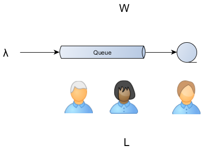
A general purpose formula, applicable to any stable system (a system where the arrival rate is not greater than the departure rate) is Little’s Law.

where

L – average number of customers
λ – long-term average arrival rate
W – average time a request spends in a system

You can apply it almost everywhere, from shoppers queues to web request traffic analysis.

This can be regarded as a simple scalability formula, for to double the incoming traffic we have two options:

1. reduce by half the response time (therefore increasing performance)
2. double the available servers (therefore adding more capacity)

A real life example

A simple example is a supermarket waiting line. When you arrive at the line up you must pay attention to the arrival rate (e.g. λ = 2 persons / minute) and the queue length (e.g. L = 6 persons) to find out the amount of time you are going to spend waiting to be served (e.g. W = L / λ = 3 minutes).

A provisioning example

Let’s say we want to configure a connection pool to support a given traffic demand.
The connection pool system is characterized by the following variables:

Ws = service time (the connection acquire and hold time) = 100 ms = 0.1s
Ls = in-service requests (pool size) = 5

Assuming there is no queueing (Wq = 0):

Our connection pool can deliver up to 50 requests per second without ever queuing any incoming connection request.

Whenever there are traffic spikes we need to rely on a queue, and since we impose a fixed connection acquire timeout the queue length will be limited.

Since the system is considered stable the arrival rate applies both to the queue entry as for the actual services:

This queuing configuration still delivers 50 requests per second but it may queue 100 requests for 2 seconds as well.

A one second traffic burst of 150 requests would be handled, since:

• 50 requests can be served in the first second
• the other 100 are going to be queued and served in the next two seconds

The timeout equation is:

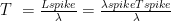
So for a 3 seconds spike of 250 requests per second:

λspike = 250requests/s
Tspike = 3s

The number of requests to be served is:

This spike would require 15 seconds to be fully processed, meaning a 700 queue buffer that takes another 14 seconds to be processed.

I'm running an online workshop on the 20-21 and 23-24 of November about High-Performance Java Persistence.

If you enjoyed this article, I bet you are going to love my Book and Video Courses as well.

Conclusion

Little’s Law operates with long-term averages and it might not suit for various traffic burst patterns. That’s why metrics are very important when doing resource provisioning.

The queue is valuable because it buys us more time. It doesn’t affect the throughput. The throughput is only sensible to performance improvements or more servers.

But if the throughput is constant then queuing is going to level traffic bursts at the cost of delaying the overflown requests processing.

FlexyPool allows you to analyze all traffic data so you’ll have the best insight into your connection pool inner workings. The fail-over strategies are safe mechanisms for when the initial configuration assumptions don’t hold on anymore.

Insert details about how the information is going to be processed

DOWNLOAD NOW